Particle Swarm Optimization
前言
粒子群优化(PSO)是罕见的能够做到编码和实现过程非常简单,同时产生奇妙的结果工具之一。 它由Eberhart和Kennedy于1995年开发的。PSO是一种生物启发式优化程序,它受到鸟类或鱼类群体的启发。它在高维,非凸,非连续的情况下表现很好。对于机器学习的超参数选择优化是个值得考虑的方法。
方法
PSO算法的主要内容可以用下面两个公式表达:
\[\vec{X_i^{t+1}} = \vec{X_i^t} + \vec{V_i^{t+1}}\] \[\vec{V_i^{t+1}} = w\vec{V_i^t} + c_1r_1(\vec{P_i^t} - \vec{X_i^t}) + c_2r_2(\vec{G^t} - \vec{X_i^t})\]这里\(t\)代表当前迭代,\(k+1\)代表下一步迭代。\(\vec{X_i^{t+1}}\)代表下一次迭代到的位置,\(\vec{V_i^{t+1}}\)代表下一次迭代的速度。使用速度来更新下一次的位置。
下一次迭代的速度\(\vec{V_i^{t+1}}\)由三部分组成:
- 惯性部分(interia term):\(w\vec{V_i^t}\)
- 个体最优部分(cognitive term):\(c_1r_1(\vec{P_i^t} - \vec{X_i^t})\)
- 全局最优部分(social term):\(c_2r_2(\vec{G^t} - \vec{X_i^t})\) 这里的\(c_1\),\(c_2\)为常数,\(r_1\),\(r_2\)为0到1的随机变量。 这意味着每一次迭代,每一个粒子都会收到自身惯性,个体最优点,全局最优点三个方向的力运动。
可以使用矢量图来解释每一个粒子的受力和最终运动方向:
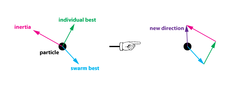 这里,能量大的粒子将继续探索新的地方。
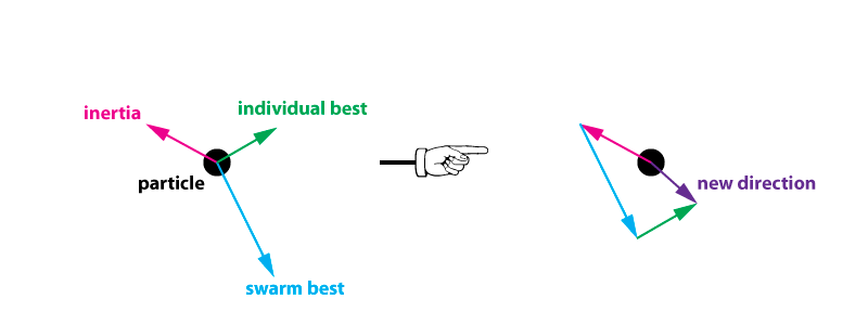 能量小的粒子会逐渐往群体靠拢。
PSO算法流程可以用如下伪代码表示:
Pseudo code of PSO

Initialize the controlling parameters (N, c1, c2, Wmin, Wmax, Vmax, and MaxIter)

Initialize the population of N particles

do
    for each particle
        calculate the objective of the particle
        Update PBEST if required
        Update GBEST if required
    end for

    Update the inertia weight
    for each particle
        Update the velocity (V)
        Update the position (X)
    end for

while the end condition is not satisified

Return GBEST as the best estimation of the global optimum
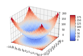
现在来看一个具体的例子:
def target(pos):
    x, y = pos
    return x*x - 10*np.cos(2*np.pi*x) + y*y - 10*np.cos(2*np.pi*y)
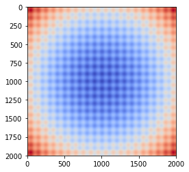
这个目标函数是我们优化的目标,可以从下面的图中看出它的最优值位于原点位置。
from mpl_toolkits.mplot3d import Axes3D
import matplotlib.pyplot as plt
from matplotlib import cm
from matplotlib.ticker import LinearLocator, FormatStrFormatter
import numpy as np

fig = plt.figure()
ax = fig.gca(projection='3d')

# Make data.
X = np.arange(-10, 10, 0.01)
Y = np.arange(-10, 10, 0.01)
X, Y = np.meshgrid(X, Y)
Z = target((X, Y))

# Plot the surface.
surf = ax.plot_surface(X, Y, Z, cmap=cm.coolwarm,
                       linewidth=0, antialiased=False)
cset = ax.contourf(X, Y, Z, zdir='z', offset=-28, cmap=cm.coolwarm)

# Customize axis
ax.set_xlim(-10, 10)
ax.set_ylim(-10, 10)

# Add a color bar which maps values to colors.
fig.colorbar(surf, shrink=0.5, aspect=5)
plt.imshow(Z, cmap='coolwarm', interpolation='nearest')
 将每一个粒子封装为一个Particle类,每个particle实例将包含粒子的速度,当前位置,最优位置,最优解误差。
class Particle:
    def __init__(self, pos, vel):
        self.pos = pos
        self.vel = vel
        self.best_pos = None
        self.best_err = float("inf")
然后,对N个粒子进行初始化,这里N取25。
# Initialize the population of N particles
N = 25
particles = []
for i in range(25):
    pos = np.random.uniform(-10, 10, size=(2,))
    vel = np.random.uniform(-1, 1, size=(2,))
    particle = Particle(pos, vel)
    particles.append(particle)

best_err_g = float("inf")
best_pos_g = None
c1 = 2
c2 = 2
w = 0.8
MaxIter = 200
初始化完毕,下面开始优化过程!
for i in range(MaxIter):
    # Main loop
    for particle in particles:
        # Calculate the objective of the particle
        err = target(particle.pos)
        # Update PBEST if required
        if err < particle.best_err:
            particle.best_err = err
            particle.best_pos = particle.pos
        # Update GBEST if required
        if err < best_err_g:
            best_err_g = err
            best_pos_g = particle.pos

    # Updatethe inertia weight
    r1 = np.random.uniform(0, 1)
    r2 = np.random.uniform(0, 1)
    for particle in particles:
        # Update the velocity
        vel_cognitive = c1*r1*(particle.best_pos - particle.pos)
        vel_social = c2*r2*(best_pos_g - particle.pos)
        particle.vel = w*particle.vel + vel_cognitive + vel_social
        # Update the position
        particle.pos = particle.pos + particle.vel
    print("Iter:{}, best_pos:{}, target:{}".format(i, best_pos_g, target(best_pos_g)))
PSO的完整的代码demo在这里,你可以运行它来看到25个粒子逐渐聚拢到最优解的动画。