Order of Growth
前言
Order of Growth 是一个根据根据函数问题大小来估算消耗计算资源上下界的方法。比如对一个list用一个循环求和会与list大小呈正比例线性关系,即使有一定的波动,它也一定会在一定的范围内。这个Order of Growth和算法本身相关。其定义为:
A method for bounding the resources used by a function by the “size” of a problem.
n: size of the problem
R(n): measurement of some resource used (time or space)
\[R(n) = \Theta(f(n))\]means that there are positive constants k1 and k2 such that:
\[k_1 \cdot f(n) \le R(n) \le k_2 \cdot f(n)\]for all n larger than some minimum m.
这里用factors和factors_fast两个简单的函数举例:要想求得一个整数n的所有factor,函数factors的方法是遍历从 1到n的所有数字,factors_fast的方法是遍历从1到\(\sqrt{n}\)的整数。后者显然循环步数更少,具体来说,它们的growth或者说复杂度分别为:
| Name | Time | Space |
|---|---|---|
| factors | \(\Theta(n)\) | \(\Theta(n)\) |
| factors_fast | \(\sqrt{n}\) | \(\sqrt{n}\) |
这两个函数的实现分别为:
from math import sqrt

def divides(k, n):
    """Return  whether k evenly divides n."""
    return n % k == 0

def factors(n):
    """Count the positive integers that evenly divide n.

    >>> factors(576)
    21
    """
    total = 0
    for k in range(1, n+1):
        if divides(k, n):
            total += 1
    return total

def factors_fast(n):
    """Count the positive integers that evenly divide n.

    >>> facotrs_fast(576)
    21
    """
    sqrt_n = sqrt(n)
    k, total = 1, 0
    while k < sqrt(n):
        if divides(k, n):
            total += 2
        k += 1
    if k * k == n:
        total += 1
    return total
可以绘图来观察steps和n的变换。下面的代码可以实现这个功能,其中repeat可以重复调用函数来计算平均时间,代码中调用的给factor的参数范围是20到10000,每次调用25取中位数然后循环后再取中位数。y轴的单位是微秒。
%matplotlib inline
import matplotlib.pyplot as plt
plt.style.use('ggplot')

from timeit import repeat
from numpy import median, percentile

def plot_times(name, xs, n=25, order=None):
    f = lambda x: name + '(' + str(x) + ')'
    g = globals()

    samples = []
    for _ in range(n):
        times = lambda x: repeat(f(x), globals=g, number=1, repeat=n)
        samples.append([median(times(x)) for x in xs])
    ys = [10e6 * median(sample) for sample in zip(*samples)]

    plt.figure(figsize=(8, 8))
    plt.plot(xs, ys)

    if order:
        slopes = [y / order(x) for (x, y) in zip(xs, ys)]
        for slope in (percentile(slopes, 0.2), percentile(slopes, 99.8)):
            plt.plot(xs, [slope * order(x) for x in xs], linewidth=3)
args = range(20, 1000)
plot_times('factors', args)
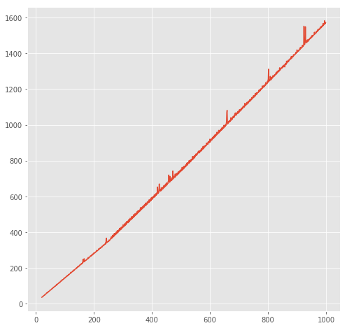
plot_times('factors_fast', args)
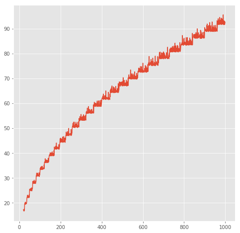
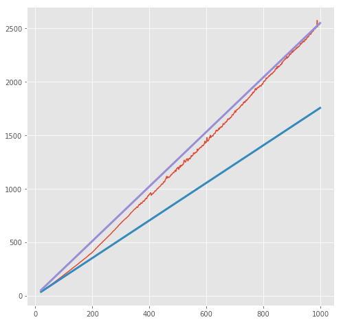
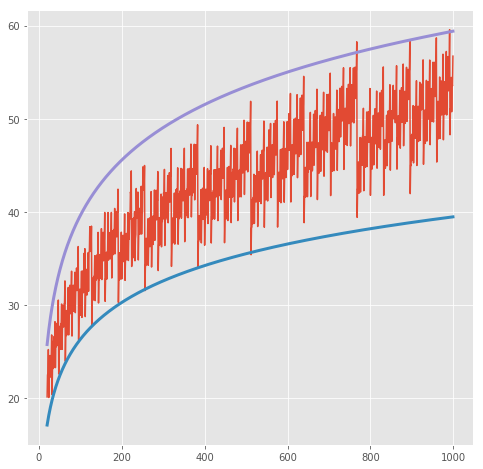
可以看到factors呈一个线性关系,而factors_fast呈一个曲线关系,我们可以画出它们的上下界:
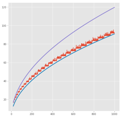
plot_times('factors', args, order=lambda x:x)
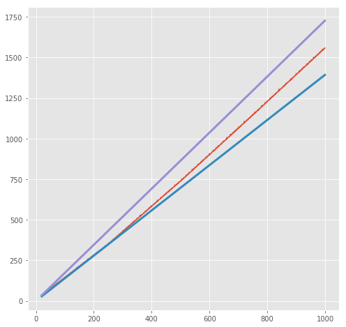
plot_times('factors_fast', args, order=sqrt)
另一个例子是exp和fast_exp。要计算一个b的n次方,exp方法是用循环从1乘到n:
\[b^n = \begin{cases} 1 & \text{if n = 0} \\ b \cdot b^{n-1} & \text{otherwise} \end{cases}\]而fast_exp使用了一个更加聪明的方法:
\[b^n = \begin{cases} 1 & \text{if n = 0} \\ (b^{\frac{1}{2}n}) ^2 & \text{if n i even} \\ b \cdot b^{n-1} & \text{if n is odd} \end{cases}\]它们的growth对比为:
| Name | Time | Space |
|---|---|---|
| exp | \(\Theta(n)\) | \(\Theta(n)\) |
| fast_exp | \(\Theta(\log(n))\) | \(\Theta(\log(n))\) |
def exp(b, n):
    """
    >>> fast_exp(2, 10)
    1024
    """
    if n == 0:
        return 1
    return b * exp(b, n-1)

def square(x):
    return x*x

def fast_exp(b, n):
    """
    >>> fast_exp(2, 10)
    1024
    """
    if n == 0:
        return 1
    elif n % 2 == 0:
        return square(fast_exp(b, n//2))
    else:
        return b * fast_exp(b, n-1)
from functools import partial
pexp = partial(exp, 2)
pfast_exp = partial(fast_exp, 2)
同样的,我们可以画出它们的曲线和上下界:
plot_times('pexp', args, order=lambda x:x)
from numpy import log
plot_times('pfast_exp', args, order=log)
Comparing orders of growth (n is the problem size)
下面是一些经典的order of growth:
- \(\Theta(b^n)\): Exponential growth, recursive fib takes \(\Theta(\phi^n)\) steps, where \(\phi = \frac{1+\sqrt{5}}{2} \approx 1.61828\). Incrementing the problem scales R(n) by a factor
- \(\Theta(n^2)\): Quadratic growth, E.g., overlap, Incrementin n increases R(n) by the problem size n.
- \(\Theta(n)\): Linear growth, E.g., slow factors or exp
- \(\Theta(\sqrt{n})\): E.g., fast factors
- \(\Theta(\log n)\): Lograithmic growth, E.g., fast exp. Doubling the problem only increments R(n).
- \(\Theta(1)\): Constant. The problem size doesn’t matter