从Data Cleaning到Model Stacking
前言
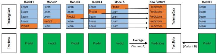
堆叠(也称为元组合)是用于组合来自多个预测模型的信息以生成新模型的模型组合技术。通常,堆叠模型(也称为二级模型)因为它的平滑性和突出每个基本模型在其中执行得最好的能力,并且抹黑其执行不佳的每个基本模型,所以将优于每个单个模型。因此,当基本模型显著不同时,堆叠是最有效的。关于在实践中怎样的堆叠是最常用的,这里我使用titanic数据集为例, 从实战出发来帮助理解。
首先读入数据:
train = pd.read_csv('titanic_train.csv')
train.head()
通过观察heatmap可以发现这里存在大量缺失的数据。
sns.heatmap(train.isnull(),yticklabels=False,cbar=False,cmap='viridis')
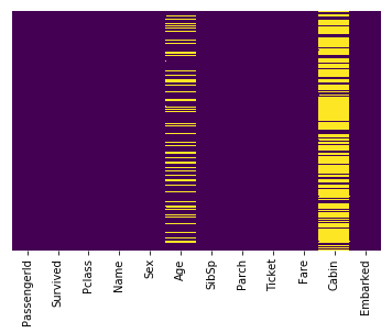
可以发现大约20%的Age数据已经缺失, 在这个缺失比例下使用imputation技术对数据进行填充是非常合理的。而对于Cabin一列,可以看见大量的数据缺失导致不能利用这一列进行判断,这时可以选择丢弃这一列,或者将这一列变化为其它特征,比如“Cabin Known: 1 or 0”。
这里使用一种巧妙的方法填充缺失的数据,可以根据不同乘客类别的平均年龄来填充:
plt.figure(figsize=(12, 7))
sns.boxplot(x='Pclass',y='Age',data=train,palette='winter')
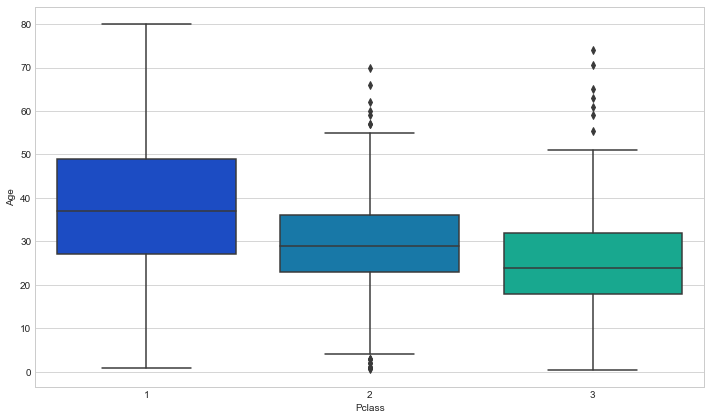
从图中可以发现更加富有的类型的乘客年龄会更大一些,这是非常合理的。然后我们可以使用这几个平均年龄来填充到Age一列。
def impute_age(cols):
    Age = cols[0]
    Pclass = cols[1]

    if pd.isnull(Age):

        if Pclass == 1:
            return 37

        elif Pclass == 2:
            return 29

        else:
            return 24

    else:
        return Age
将该函数apply到DataFrame数据结构上:
train['Age'] = train[['Age','Pclass']].apply(impute_age,axis=1)
对于Cabin一列,选择丢弃它。同时还要丢弃Embarked一列为NaN的那几行数据:
train.drop('Cabin',axis=1,inplace=True)
train.dropna(inplcae=True)
然后来检查确认一下数据中不存在缺失的数据了:
train.isnull().sum()
PassengerId    0
Survived       0
Pclass         0
Name           0
Sex            0
Age            0
SibSp          0
Parch          0
Ticket         0
Fare           0
Embarked       0
dtype: int64
转化Categorical Features
然后我们需要将类别特征(categorical features)转化为伪变量(dummy variables),否则机器学习的算法不能将它们作为输入的特征:
sex = pd.get_dummies(train['Sex'],drop_first=True)
embark = pd.get_dummies(train['Embarked'],drop_first=True)
train.drop(['Sex','Embarked','Name','Ticket'],axis=1,inplace=True)
train = pd.concat([train,sex,embark],axis=1)
train.head()
| PassengerId | Survived | Pclass | Age | SibSp | Parch | Fare | male | Q | S | |
|---|---|---|---|---|---|---|---|---|---|---|
| 0 | 1 | 0 | 3 | 22.0 | 1 | 0 | 7.2500 | 1 | 0 | 1 |
| 1 | 2 | 1 | 1 | 38.0 | 1 | 0 | 71.2833 | 0 | 0 | 0 |
| 2 | 3 | 1 | 3 | 26.0 | 0 | 0 | 7.9250 | 0 | 0 | 1 |
| 3 | 4 | 1 | 1 | 35.0 | 1 | 0 | 53.1000 | 0 | 0 | 1 |
| 4 | 5 | 0 | 3 | 35.0 | 0 | 0 | 8.0500 | 1 | 0 | 1 |
然后需要对test数据集做同样的处理。
# Impute or drop missing data
test = pd.read_csv('./titanic_test.csv')
test['Age'] = test[['Age','Pclass']].apply(impute_age,axis=1)
test.drop('Cabin',axis=1,inplace=True)
test.dropna(inplace=True)

# Convert dummpy variable
sex = pd.get_dummies(test['Sex'],drop_first=True)
embark = pd.get_dummies(test['Embarked'],drop_first=True)
test.drop(['Sex','Embarked','Name','Ticket'],axis=1,inplace=True)
test = pd.concat([test,sex,embark],axis=1)
test.head()
| PassengerId | Pclass | Age | SibSp | Parch | Fare | male | Q | S | |
|---|---|---|---|---|---|---|---|---|---|
| 0 | 892 | 3 | 22.0 | 0 | 0 | 7.8292 | 1 | 1 | 0 |
| 1 | 893 | 3 | 38.0 | 1 | 0 | 7.0000 | 0 | 0 | 1 |
| 2 | 894 | 2 | 26.0 | 0 | 0 | 9.6875 | 1 | 1 | 0 |
| 3 | 895 | 3 | 35.0 | 0 | 0 | 8.6625 | 1 | 0 | 1 |
| 4 | 896 | 3 | 35.0 | 1 | 1 | 12.2875 | 0 | 0 | 1 |
Model Stacking
所有的数据都已经准备就绪,下面进行正式开始模型融合。
X_train = train.drop('Survived', axis=1)
y_train = train['Survived']
X_test = test
from sklearn.model_selection import KFold
import numpy as np

ntrain = train.shape[0] #891
ntest = test.shape[0] # 418
kf = KFold(n_splits=5, random_state=666)
from sklearn.linear_model import LogisticRegression
logmodel = LogisticRegression()
# Get out-of-folder
def get_oof(clf, X_train, y_train, X_test):
    oof_train = np.zeros((ntrain,))
    oof_test = np.zeros((ntest,))
    oof_test_skf = np.empty((5, ntest))

    for i, (train_index, test_index) in enumerate(kf.split(X_train)): # X_train: 891 * 7
        kf_X_train = X_train.iloc[train_index] # 712 * 7 ex: 712 instances for each fold
        kf_y_train = y_train.iloc[train_index] # 712 * 1 ex: 712 instances for each fold
        kf_X_test = X_train.iloc[test_index] # 179 * 7 ex: 178 instances for each fold

        clf.fit(kf_X_train, kf_y_train)

        oof_train[test_index] = clf.predict(kf_X_test) # 1 * 179 =====> will be 1 * 891 after 5 folds
        oof_test_skf[i, :] = clf.predict(X_test) # oof_test_skf[i, :]: 1 * 418

    oof_test[:] = oof_test_skf.mean(axis=0) # oof_test[:] 1 * 418
    return oof_train.reshape(-1, 1), oof_test.reshape(-1, 1)
oof_train, oof_test = get_oof(logmodel, X_train, y_train, X_test)
oof_train.shape
(889, 1)
oof_test.shape
(418, 1)